Pierre-Simon Laplace was one of the earliest thinkers who had considered celestial forces as a result of a fluid flow of some sort. He has written the following :
“If gravitation be produced by the impulse of a fluid directed towards the centre of the attracting body, the preceding analysis… will give the secular equation depending on the successive transmission of the attractive force.”.
This blog is about trying to understand various classical and perhaps quantum phenomena found in nature by utilizing a fluid flow analogy. To be more exact , in modern terms, I’m thinking of an analogy stemming from the field of continuum mechanics, and various phenomena therein.
I will show how electricity can be seen as an internal friction in the space-time fluid flow. This is work in progress, so I do not know yet what I will end up with.
Most of the physical laws are related somehow to the idea of conservation of things. For example, one has the conservation of linear momentum, conservation of angular momentum and so forth. Of course we also have the conservation of energy principle, which is probably the most intuitive in a prosaic sense. Usually these mathematical statements then produce in one way or another some mathematical equations that represent e.g. Newtons’s laws of motion.
The other very popular approach is the dynamic optimization paradigm, where one sees the mother nature as an optimal controller of some sort, where typically some functional is to be minimized over a path. The optimality conditions (Euler-Lagrange equations) then usually resemble Newton’s laws of motion again. Analogically, one has for example in the field of economics some behavioral laws in the same spirit.
This all is physics from the 19th century, before Einstein and before the quantum revolution. Personally I find two ontological issues with 20th century physics: the first one is my lack of understanding what quantum physics really is. In other words, I fail to find a reasonable explanation why energy and momentum can be represented through differential operators in Hilbert space. The second problem I have is that I basically do not think that General Relativity is ontologically correct. I do not like the idea of curved space.
From these rather unpleasant feelings, I began to think of some new ways to describe some rather basic concepts in physics. I became fascinated with fluids, as the mathematics of fluids is extremely complicated and therefore allow for rich behavior. First and foremost: fluid mechanics is non-linear. This makes things hard.
In my opinion, fluids have three main features that are especially important
1) The vorticity of the fluid (curls and eddies, spirals)
2) The compressibility of fluids
3) The viscosity properties of fluids (friction, like water vs. oil)
So I started to think about fluids of space-time. Moreover, even though I do not like the ideas of General Relativity, I think that the incorporation of time in the coordinate space is essential. To have a nice theory or a model, we must have solid assumptions. My assumption of the form of space-time is the following (Poincaré, Minkowski): the coordinate vector is

So that we have the three usual spatial coordinates and one imaginary time-component. This inclusion of the imaginary unit is nice, because we can see directly that inner product has the correct form

This inclusion of the imaginary unit gives also rise directly to the following differential operator (just think of partials with respect to space-time coordinates):

So. Great. We have a 4D nabla operator and a space. Let’s play around. We need some more ingredients, though. Drawing ideas from the potential representation of Maxwell’s equations, let us define a 4-potential:

The potentials can take values in the complex field, but for now it is okay to think of them as functions from space and time to the real numbers.
We now make a brief incursion to the ideas of conservation of energy. The total energy of a system (called the Hamiltonian) is composed of the potential energy of the system and of the kinetic energy of the system. Energy is usually thought as a real number like “3 kilo-watt-hours”. I’m extending the concept of energy into matrix values. So potential energy is a matrix and kinetic energy is a matrix. The total energy is therefore simply the sum of these matrices. In symbols:

The matrices are 4 times 4 square matrices. Moreover, I require them to be symmetric. Symmetry is beautiful and symmetric matrices have lots of nice properties (like real eigenvalues). Moreover, symmetry of the matrices is related to the conservation of angular momentum.
So we have the most basic equation at hand. Statement of total energy. We need to add some structure in order to build a meaningful model.
Let us start by thinking of kinetic energy. Usually it is something involving velocity squared. So we need velocities. Here is the crucial assumption: let us think of the 4-potential as a 4-velocity field. The natural way to induce a square matrix from the 4-velocity is to take the outer product of the “velocities” as follows:
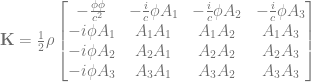
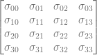
So this is the kinetic energy matrix of our fluid in space-time. In a similar manner, we need to define the potential energy matrix. This is trickier, as we need a symmetric matrix which meaningfully represents potential energy. Well, we can steal some ideas from continuum mechanics. In continuum mechanics, the potential is related to pressure and frictional forces, which can be summarized in the so-called Cauchy Stress Tensor :

where the so-called deviatoric (first term on the right side) part is defined as
The second term is just pressure function times an identity matrix.
Now, obviously at this time, the stress tensor is just a collection of symbols.
The most general form which retains symmetry and has dependence on the space-time velocity gradient is the following:

We can however add more structure by assuming that the frictional forces are linear in the gradient of the velocity field. This constitutes a Newtonian fluid. One can think of this as two layers of fluid moving next to each other, the friction is produced by the velocity differences, think of rubbing your hands together.
This Newtonian fluid assumption can be stated compactly by saying
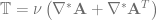
The matrix is obviously symmetric, as if you add the transpose, this does the trick.
So in the end we have the most general equation

This equation will conclude my first posting on this topic. In the next post I will show how electricity is the friction in this space-time fluid.
