The main philosophical question that is at the root of the fluid model presented here is the following: what is the ontological meaning of the four potential 
As I explained earlier, the most important properties of fluids are the divergence, vorticity and viscosity (which are interrelated). I have already shown that the divergence of the fluid is directly linked to the Lorentz-gauge and that the vorticity of the fluid is essentially the electromagnetic field tensor. What occurred to me recently was the concept of “curvature”. Now curvature is important, as the general relativity describes that mass and energy alter the curvature of the space (i.e. the metric tensor differs from the Kronecker delta). Curvature is a nice heuristic concept more generally as well, because for example we can describe the flow of heat using the heat equation based on the curvature of the temperature field. Similarly, electrostatics and Newtonian gravity are based essentially on Poisson’s equation where charge or mass generate curvature on the potential. So I started thinking about curvature of the velocity field of aether.
So what is curvature? As a first approximation we can understand it through the second derivative or the Laplacian. In differential geometry we have concepts like the Riemann tensor, Ricci tensor and so forth. However, as I want to keep things as simple as possible, I start of with the Laplacian approach, which actually takes me quite far as you shall see. Let us then consider a 3-dimensional space and take the following vector calculus identity

This is a beautiful identity as it binds together the “curvature” and divergence of the vector field, which together manifest themselves as the curl of the curl of the vector field. What I realized, was that this actually means that the curl of the curl is basically a commutator, i.e. it measures how much the divergence and gradient do not commute locally. Not to mention that this is actually quite close to the definition of the Riemann tensor!
Now I shall the construct a curvature concept for the aether fluid. This is straightforward, but it is rather complicated in 4-dimensions, because the curl operator has to be generalized as I’ve done in my earlier posts. Nevertheless, the end result is a rank 3 tensor, which has 64 components.
I began my interest in this curl of the curl concept also because of some experiments that have to do with rotating magnetic fields. Nikola Tesla was one of the pioneers in the field. Apparently rotating magnetic fields can produce quite interesting effects which have to do with gravity. See for example the following article by the European Space Agency
Obviously it is also quite interesting that the rotation of the magnetic field happens to be linked to the curl of curl of the vector potential! So curvature, rotating magnetic fields and gravitation are all linked together in some mysterious way.
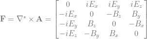
Let us then find what is the “curvature” of the “aether” field. What we already have is the curl of the velocity field, which I obtained using the sort of exterior/Grassmann algebra:

We can state this in a more simple notation using the symbols for electric and magnetic field
How to then apply the curl to a second rank tensor? We can do it by proceeding to each column vector separately. First we take the column vector and form a gradient tensor out of it. The first column vector is

So that the gradient tensor is
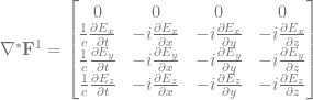
One should note btw that the diagonal contains the divergence of the electric field.
In similar manner, one has the second column vector,

What one needs to do then is to take the transpose of the each gradient tensors and take the difference of the gradient tensor and its transpose. The result is a rank 3 tensor which contains just so much information that it needs another posting…
